Pivot Table

Tough

How do we do cross conditional formating in a pivot table on a dimension column based on measures?

eg I have a report which should display
Pivot Table1 - year , month, date, revenue - no conditional formatting
Pivot table2 - year in rows, month in column and revenue in measures with cross conditional formatting column - year. The Conditions are
revenue less than 15000 - red colour
revenue greater than 30000 - blue colour
revenue between 15000 and 30000 - pink colour.

Create a report with columns year,month,date,revenue

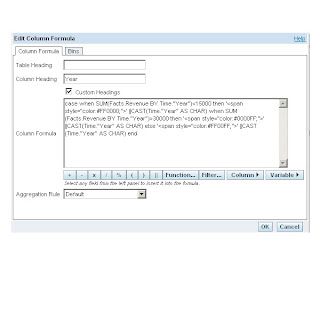
Conditional Formatted Column formula



go to the Format tab of the first column and go to Data Format
check the check box of Override Default Data Format
and select HTML from the drop down

Create the pivot table 1 with year(second column) ,month, date and revenue
pivot table2 with year(first column) in rows, month in columns and revunue in measures

This report should have atleast 3 columns.We are actually creating a pivot table metrics Facts.Revenue at year level in a report formula which can be done by a report calculated level based measure (SUM(Facts.Revenue BY Time."Year"). Then we are comparing with the conditions and we are concatinating the HTML Colour tag(<span >). Here it should be noted that (SUM(Facts.Revenue BY Time."Year") less than 15000 is the conditional part aand the HTML Colour tag is the formating part. The Actual Report should have the column Time."Year" pulled in the report, if it is not required hide it.

This shows one of the method of cross conditional formating in a pivot table on a dimension column based on measures

How do we do cross conditional formating in a pivot table on a fact column based on dimensions?

Eg I have a report with month from target date, month from completed date. All the measures in the pivot table which are completed on or before the target month should have back ground colour as green and remaining as red.we also need a table view with the above colmns and the completed date.

Create a report with columns month from target date, month from completed date, measures and completed date.

Conditional Formatted Column formula



Go to the Format tab of the first column and go to Data Format check the check box of Override Default Data Format and select HTML from the drop down



Create the pivot table as shown in the figure

In addition to the explanation mentioned in the above question , it should be noted that we are putting an aggregation to convert a text field to measures in pivot table.

This shows one of the method of cross conditional formating in a pivot table on a fact column based on dimensions.